Visualizing Data
This notebooks shows examples of how to visualize data using the Holoviews and hvplot libraries with both xarray and pandas. Additional information can be found in the Holoviews user guide.
Open an interactive notebook:
Sign into the SHIFT SMCE Daskhub and select an instance size in a different tab
Follow this link
Select the “notebook” kernel
import sys
sys.path.append('/efs/SHIFT-Python-Utilities/')
from shift_python_utilities.intake_shift import shift_catalog
import xarray as xr
import rioxarray as rxr
import math
import numpy as np
import holoviews as hv
from holoviews.plotting.links import DataLink
from holoviews import opts, streams
hv.extension('bokeh')
import pandas as pd
import hvplot.pandas
pd.options.plotting.backend = 'holoviews'
import hvplot.xarray
# Supporting functions

def gamma_adjust(array):
    # Rescale Values using gamma to adjust brightness
    # Create exponent for gamma scaling - can be adjusted by changing 0.2
    gamma = math.log(0.2)/math.log(np.nanmean(array))

    # Apply scaling and clip to 0-1 range
    scaled = np.power(array,gamma).clip(0,1)

    #Assign NA's to 1 so they appear white in plots
    scaled = np.nan_to_num(scaled, nan = 1)
    return scaled

def find_nearest(array1, array2):
    new_array = np.zeros(array2.shape)

    for ind, value in enumerate(array2):
        idx = (np.abs(array1 - value)).argmin()
        new_array[ind] = array1[idx]

    return new_array
# Read in the data using the shift python utilities library
cat = shift_catalog()
ds = cat.aviris_v1_gridded.read_chunked()

# Data can also be oppened using xarray
# ds = xr.open_dataset("reference://", engine="zarr", backend_kwargs={
#     "consolidated": False,
#     "storage_options": {"fo": "s3://dh-shift-curated/aviris/v1/gridded/zarr.json"}
# })

# Data can be oppened using rioxarray, however the xarray coordinates and data variables might use different names
# ds = rxr.open_rasterio("/efs/efs-data-curated/v1/20220308/L2a/ang20220308t184127_rfl")

# Subset the data using the select method
aoi = ds.sel(x=slice(730300,731000), y=slice(3819660,3819050), time="2022-03-08")
aoi

Plotting an RGB image
# Retreive red, green and blue wavelengths and convert them to numpy arrays
red = aoi.sel(wavelength=650, method="nearest").reflectance
green = aoi.sel(wavelength=560, method="nearest").reflectance
blue = aoi.sel(wavelength=470, method="nearest").reflectance

# Scale the Bands
r = gamma_adjust(red)
g = gamma_adjust(green)
b = gamma_adjust(blue)

# Stack Bands and make an index
rgb = np.stack([r,g,b])
bds = np.array([0,1,2])

# Pull x and y values
y = aoi['y'].values
x = aoi['x'].values

# Stack Bands and make an index
rgb = np.stack([r,g,b])
bds = np.array([0,1,2])

# Pull x and y values
y = aoi['y'].values
x = aoi['x'].values

# Create new rgb xarray data array.
data_vars = {'RGB':(['wavelength','y','x'], rgb)}
coords = {'wavelength':(['wavelength'],bds), 'y':(['y'],y), 'x':(['x'],x)}
attrs = aoi.attrs
ds_rgb = xr.Dataset(data_vars=data_vars, coords=coords, attrs=attrs)
ds_rgb.coords['x'].attrs = aoi['x'].attrs
ds_rgb.coords['y'].attrs = aoi['y'].attrs
ds_rgb

# Create the RGB Image
rgb_image = ds_rgb.hvplot.rgb(x='x', y='y', bands='wavelength',
                              aspect='equal', frame_width=400).opts(tools=["hover"])
rgb_image

Using Holoviews with a Pandas Dataframe
# Generate some random data
data = np.random.randn(1000,2 )

# Create a Pandas Dataframe with the data
df = pd.DataFrame({'x': data[:, 0], 'y': data[:, 1]})

# Create a scatterplot with the data, specifying the desired tools
points = df.hvplot.scatter(x="x", y="y", width=400, height=400).opts(
    tools=["hover", "lasso_select", "box_select"])

# Create a table from the scatter plot
table = hv.Table(points)

# Create a stream
sel = hv.streams.Selection1D(source=points)

# Define a function to be used by the stream
def selected_info(index):
    return hv.Table(points.iloc[index], kdims=['index'], vdims=['x', 'y'])

# Access the selected data
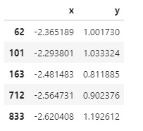
df.iloc[sel.index]
Using Holoviews with Xarray
Selecting a Subset of an Image
# Create the RGB image plot
rgb_image = ds_rgb.hvplot.rgb(
    x='x', y='y', bands='wavelength', aspect = 'equal', frame_width=400).opts(
    tools=["hover", 'box_select'])

# Create our data stream for the box selection
sel = hv.streams.BoundsXY(source=rgb_image, bounds=(0,0,0,0))

# Create a function to process the selection
def selected_info(bounds):
    mask = (
        (ds_rgb.coords["x"] >= bounds[0])
        & (ds_rgb.coords["x"] <= bounds[2])
        & (ds_rgb.coords["y"] >= bounds[1])
        & (ds_rgb.coords["y"] <= bounds[3])
    )

    return xr.where(~mask, 1., ds_rgb['RGB']).transpose('wavelength', 'y', 'x').hvplot.rgb(
        x='x', y='y', bands='wavelength', aspect = 'equal', frame_width=400)

# Create a dynamic map using the function and stream
box = hv.DynamicMap(selected_info, streams=[sel])
#Plot both the RGB image and our dynamic map
(rgb_image + box)
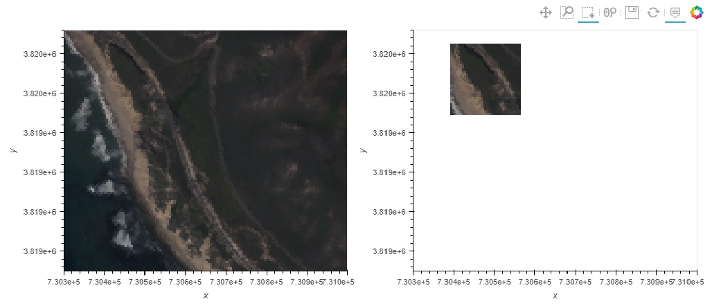
b = box.streams[0].bounds
ds_rgb.sel(x=slice(b[0], b[2]), y=slice(b[3], b[1])).hvplot.rgb(
    x='x', y='y', bands='wavelength', aspect='equal')

Spectra Selection
# Create the RGB image plot
rgb_image = ds_rgb.hvplot.rgb(
    x='x', y='y', bands='wavelength', aspect = 'equal', frame_width=400).opts(
    tools=["hover", 'lasso_select'])

# Create streams
posxy = hv.streams.PointerXY(source=rgb_image, x=730302.5, y=-3819657.5)
sel = hv.streams.Lasso(source=rgb_image, geometry=np.array([[730302.5, 3819657.5]]))

# Function to build a new spectral plot based on mouse hover positional
# Information retrieved from the RGB image using our full reflectance dataset
def point_spectra(x,y):
    return aoi.sel(x=x,y=y,method='nearest').hvplot.line(
        y='reflectance',x='wavelength', color='#1b9e77', frame_width=400)

def selected_info(geometry):
    x = find_nearest(aoi.x, geometry[:, 0])
    y = find_nearest(aoi.y, geometry[:, 1])
    points = set(list(zip(x, y)))

    list_of_lines = [aoi.sel(x=x, y=y, method='nearest').hvplot.line(
        y='reflectance',x='wavelength', frame_width=400) for x, y in points]
    return hv.Overlay(list_of_lines)

# Define the Dynamic Maps
point_dmap = hv.DynamicMap(point_spectra, streams=[posxy])
lasso_dmap = hv.DynamicMap(selected_info, streams=[sel])

# Plot the RGB image and Dynamic Maps side by side
(rgb_image + point_dmap*lasso_dmap)
