Loading SHIFT Data with Intake
The SHIFT Python Utilities library has a custom intake driver which provides a simple interface for reading in SHIFT data. The custom driver allows for common preprocessing operations such as orthorectifying and subseting with a bounding box or shapefile.
This notebook demonstrates some of the basic xarray functionality.
Open an interactive notebook:
Sign into the SHIFT SMCE Daskhub and select an instance size in a different tab
Follow this link
Select a kernel
import math
import numpy as np
import matplotlib.pyplot as plt
import xarray as xr
import pandas as pd
import os
os.environ['USE_PYGEOS'] = '0'
import geopandas as gpd
import hvplot.pandas
import sys
sys.path.append('/efs/SHIFT-Python-Utilities/')
from shift_python_utilities.intake_shift import shift_catalog
import holoviews as hv
hv.extension('bokeh')
import hvplot.xarray
from sklearn.decomposition import PCA
from sklearn.cluster import KMeans
import warnings
warnings.filterwarnings("ignore")
# Supporting Functions
def gamma_adjust(array):
    # Rescale Values using gamma to adjust brightness
    gamma = math.log(0.2)/math.log(np.nanmean(array)) # Create exponent for gamma scaling - can be adjusted by changing 0.2
    scaled = np.power(array,gamma).clip(0,1) # Apply scaling and clip to 0-1 range
    scaled = np.nan_to_num(scaled, nan = 1) #Assign NA's to 1 so they appear white in plots
    return scaled

def generate_rgb_plot(ds):
    # Retreive red, green and blue wavelengths and convert them to numpy arrays
    red = ds.sel(wavelength=650, method="nearest").reflectance
    green = ds.sel(wavelength=560, method="nearest").reflectance
    blue = ds.sel(wavelength=470, method="nearest").reflectance

    # Scale the Bands
    r = gamma_adjust(red)
    g = gamma_adjust(green)
    b = gamma_adjust(blue)

    # Stack Bands and make an index
    rgb = np.stack([r,g,b])
    bds = np.array([0,1,2])

    rgb.shape
    # Pull x and y values
    y = ds['lat'].values
    x = ds['lon'].values
    y.shape
    x.shape
    rgb.shape
    # Create new rgb xarray data array.
    data_vars = {'RGB':(['wavelength', 'lat', 'lon'], rgb)}
    coords = {'wavelength':(['wavelength'],bds), 'lat':(['lat'],y), 'lon':(['lon'],x)}
    attrs = ds.attrs
    ds_rgb = xr.Dataset(data_vars=data_vars, coords=coords, attrs=attrs)
    ds_rgb.coords['lon'].attrs = ds['lon'].attrs
    ds_rgb.coords['lat'].attrs = ds['lat'].attrs

    return ds_rgb
# Open the data catalog
cat = shift_catalog()
# List available datasets
cat.datasets
[‘aviris_v1_gridded’, ‘L2a’, ‘L1’]
# List child datasets
cat.L1.datasets
[‘glt’, ‘igm’, ‘obs’, ‘rdn’]
Reading in Data
Data can be read in using two function calls: read and read_chunked. The read method will pull all the data in the dataset into memory. It is highly recommended to use the read_chunked method unless you are sure your data can fit into memory.
data = cat.aviris_v1_gridded.read_chunked()
data

Working with L1 and L2a Data
The L1 and L2a data products can be accessed via the catalog. To load a specific file, use date and the time of the flight. A list of possible dates and times can be retrieved using the following code. The data is located /efs/efs-data-curated. In addition to date and time there are several other arguments you can use to preprocess the data.
Optional Arguments:
ortho (bool, default: False): If set to True, the associated GLT file will be used to orthorectify the dataset. Warning orthorectification is a very memory intensive process and depending on the size of the file the Daskhub may not have enough memory to complete the task. In this case you can use the SHIFT cluster or use the subsetting argument to orthorecticy a section of the dataset
filter_bands (bool, default: False)(np.ndarray or list): For this argument you can pass a boolean and it will use a set mask to filter out bands. Additionally, if you would like to use a custom mask, you can pass an array or list with the indicies of bands you would like filtered.
Here is a list of the default filtered bands:
[1, 2, 3, 194, 195, 196, 197, 198, 199, 200, 201, 202, 203, 204, 205, 206, 207, 208, 209, 210, 211, 212, 213, 214, 215, 216, 217, 286, 287, 288, 289, 290, 291, 292, 293, 294, 295, 296, 297, 298, 299, 300, 301, 302, 303, 304, 305, 306, 307, 308, 309, 310, 311, 312, 313, 314, 315, 316, 317, 318, 319, 320, 321, 322, 323, 324, 325, 326, 327, 328, 329, 330, 331, 332, 333, 334, 335, 415, 416, 417, 418, 419, 420, 421, 422, 423, 424, 425]
subset (dict, GeoDataFrame, default: None): This argument allows you to subset the dataset by index(x, and y), latitude and longitude, or with a shapefile formatted as a GeoPandas Dataframe. If using a shapefile, the ortho argument must be set to True.
chunks (dict, default: {‘y’: 1}): This argument controls how dask chunks up your array. I recommend using the default of chunking along the y dimension however, depending on what your computing, chunking differently my increase the performance.
# List the available dates
cat.dates
[‘20220224’, ‘20220228’, ‘20220308’, ‘20220316’, ‘20220318’, ‘20220322’, ‘20220405’, ‘20220412’, ‘20220420’, ‘20220429’, ‘20220503’,’20220511’,’20220512’, ‘20220517’, ‘20220529’, ‘20220914’, ‘20220915’]
# Use a date to get the available times
cat.times["20220228"]
[‘183924’, ‘185150’, ‘185720’, ‘190702’, ‘192104’, ‘193333’, ‘194708’, ‘195958’, ‘201833’, ‘202944’, ‘204228’, ‘205624’, ‘210940’, ‘212724’, ‘214527’, ‘215349’]
# Use a date and a time to retrieve the L2a file
cat.L2a(date="20220228", time="183924").read_chunked()

# Use a date and a time to retrieve the radiance file
cat.L1.rdn(date="20220228", time="183924").read_chunked()

Orthorectifying a Dataset
Using the GLT file
In order to orthorectify a dataset using the GLT file, all you need to do is set the ortho argument to True.
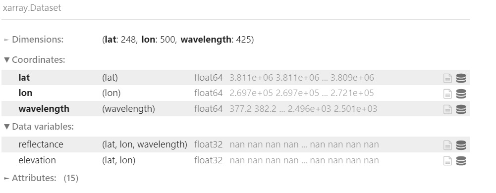
ds = cat.L2a(date="20220228", time="183924", ortho=True, filter_bands=False).read_chunked()
ds

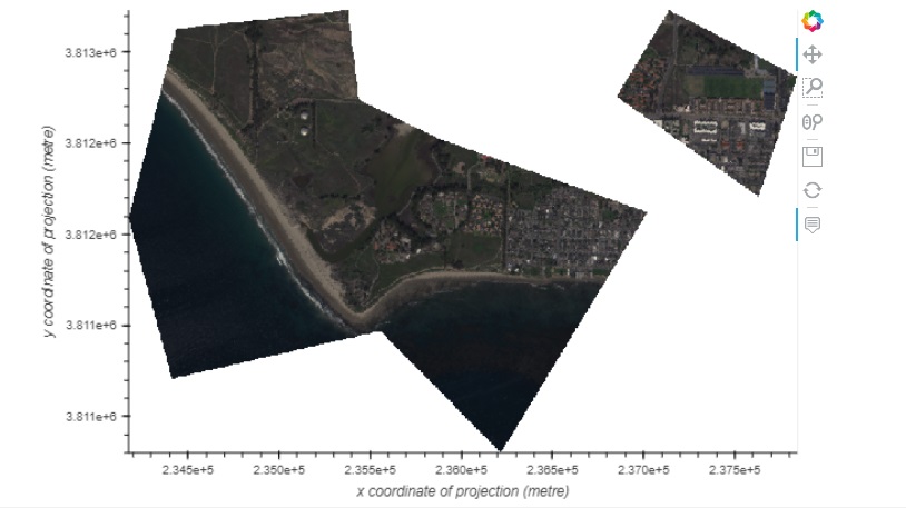
Now that the data is orthorectified we can plot an RGB image of the scene.
ds_rgb = generate_rgb_plot(ds)
rgb_image = ds_rgb.hvplot.rgb(x='lon', y='lat', bands='wavelength', aspect = 'equal', frame_width=600).opts(tools=["hover"])
rgb_image

Orthorectifying a Subset of a File
Many of the SHIFT reflectance and radiance files are too large to orthorectify the entire scene. Using the subset argument a portion of the scene can be selected and orthorectified. As described above the subset argument can be used with:
x and y indicies
lat and lon values (using the correct CRS)
A shapefile formated as a GeoPandas dataframe (using the correct CRS)
Orthorectifying using x and y indicies
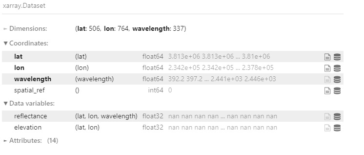
ds = cat.L2a(date="20220228", time="183924", ortho=True, filter_bands=True, subset={'x':slice(29, 200), 'y':slice(34, 500)}).read_chunked()
ds
ds_rgb = generate_rgb_plot(ds)
rgb_image = ds_rgb.hvplot.rgb(x='lon', y='lat', bands='wavelength', aspect = 'equal', frame_width=600).opts(tools=["hover"])
rgb_image

Orthorectifying using lat and lon
eastings = np.array([228610.68861488, 237298.11871802])
northings = np.array([3812959.0852389 , 3810526.08057343])
ds = cat.L2a(date=20220224, time=200332, ortho=True, filter_bands=True, subset={'lat':northings, "lon": eastings}).read_chunked()
ds

ds_rgb = generate_rgb_plot(ds)
rgb_image = ds_rgb.hvplot.rgb(x='lon', y='lat', bands='wavelength', aspect = 'equal', frame_width=600).opts(tools=["hover"])
rgb_image

Orthorectifying using a shapefile
shp = gpd.read_file("~/SHIFT-Python-Utilities/shift_python_utilities/tests/test_data/shp/test.shp")
ds = cat.L2a(date=20220224, time=200332, ortho=True, filter_bands=True, subset=shp).read_chunked()
ds
ds_rgb = generate_rgb_plot(ds)
rgb_image = ds_rgb.hvplot.rgb(x='lon', y='lat', bands='wavelength', aspect = 'equal', frame_width=600).opts(tools=["hover"])
rgb_image
Using the IGM File
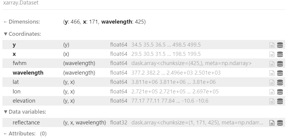
For this section we set the ortho argument to false and use the lat and lon data from the igm file to orthorectify outputs.
# Retrieve a subset of a scene
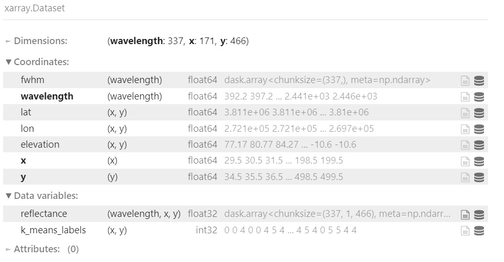
ds = cat.L2a(date="20220228", time="183924", ortho=False, filter_bands=True, subset={'x':slice(29, 200), 'y':slice(34, 500)}).read_chunked()
ds
Use the Lat and Lon values to plot an orthorectified elevation map.
# Load the lat, lon and elevation values into memory
x = ds.lon.values
y = ds.lat.values
z = ds.elevation.values
# Create a contour plot using matplotlib
fig,ax=plt.subplots(1,1, figsize=(20, 6))
cp = ax.contourf(x, y, z, levels=15)
fig.colorbar(cp) # Add a colorbar to a plot
ax.set_title('Elevation Map')
plt.show()

Use the lat and lon values to plot a classification map of the scene.
# Combine the x and y dimension to format data for the PCA
ds = ds.stack(combined=('x', 'y'))
pca = PCA(n_components=3).fit(ds.reflectance.values)

# Perform clustering using the PCA outputs
kmeans = KMeans(n_clusters=6, init = 'k-means++', random_state=42)
kmeans = kmeans.fit(pca.components_.T)

# Add the clustering labels to the dataset as a new variable
ds = ds.assign({'k_means_labels':(['combined'], kmeans.labels_)})

# Return the dataset to its original shape by unstacking the x and y dimensions
ds = ds.unstack('combined')
ds
# Use the hvplot quadmesh plot to create the classification map
classification_map = ds.k_means_labels.hvplot.quadmesh(x='lon', y='lat')
classification_map
