Aligning Field and SHIFT Data
import pandas as pd
 import geopandas as gdp
 import rioxarray as rxr
 import xarray as xr
 import rasterio as rio
 import numpy as np
 import sys
 sys.path.append('/efs/SHIFT-Python-Utilities/')
 from shift_python_utilities.intake_shift import shift_catalog
 from joblib import Parallel, delayed
 import holoviews as hv
 hv.extension('bokeh')
 import hvplot.xarray

 cat = shift_catalog()
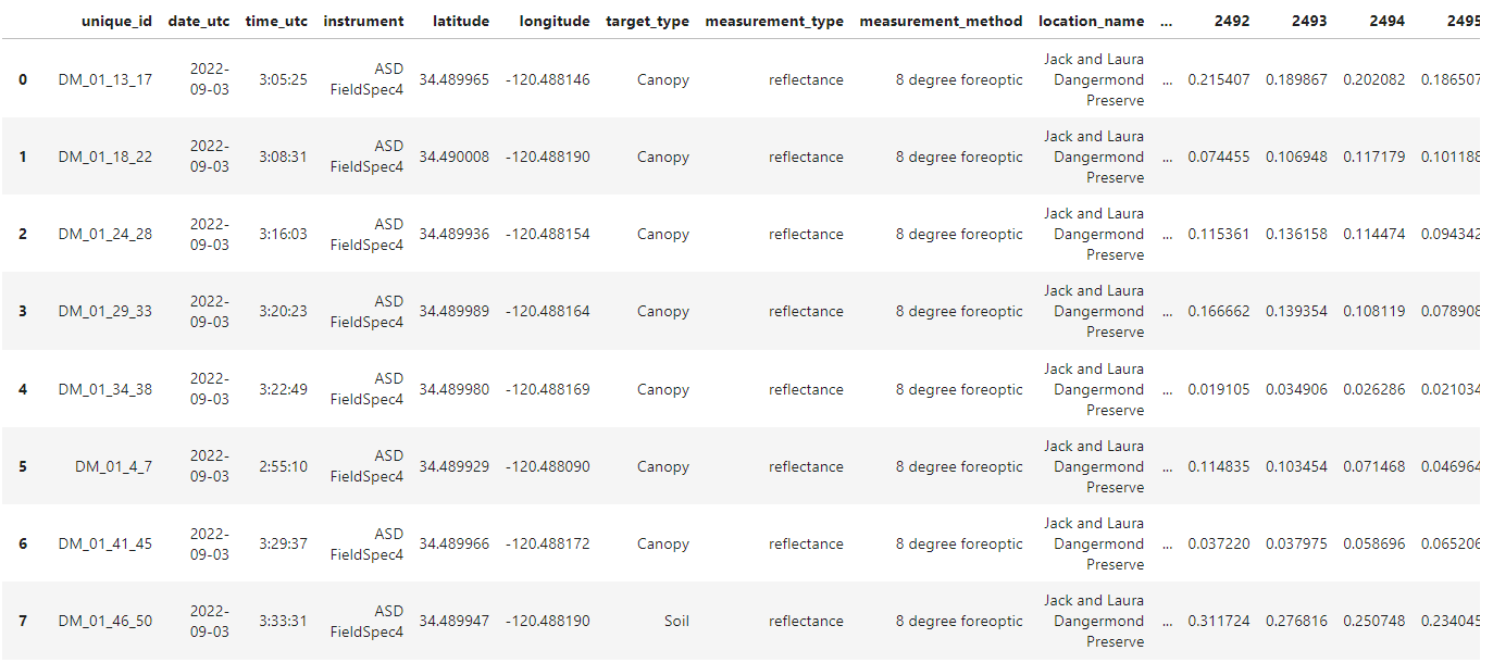
Read in our field data csv using Pandas
Convert the dataframe to a Geopandas dataframe using the latitudes and longitudes
Remove sites missing lattitudes and longitudes
Filter sites by target type. For this dataset we are only interested in the soil and canopy targets
df = pd.read_csv('/efs/edlang1/FieldData_yangello_DAAC.csv')

gdf = gdp.GeoDataFrame(
    df, geometry=gdp.points_from_xy(df.longitude, df.latitude), crs="EPSG:4326"
)

# Filter out sites missing lat/lon values
gdf = gdf[~np.isnan(np.asarray(gdf.latitude))].reset_index(drop=True)

# Filter by target type
gdf = gdf[(gdf.target_type == 'Canopy') | (gdf.target_type == "Soil")].reset_index(drop=True)
gdf
Georeference our SHIFT data
ds = cat.aviris_v1_gridded().read_chunked()
ds.rio.write_crs(rio.CRS.from_wkt(",".join(ds.attrs['coordinate system string'])), inplace=True)
ds.rio.crs
Our field sites are 30 by 30 meter grids:
Convert the geodataframe’s CRS to UTM so it is meter based instead of degrees.
Using Shapely, create a 15 meter square (cap_style of 3) buffer around our field sites.
gdf = gdf.to_crs(gdf.estimate_utm_crs())
# create a 30 by 30 square around each point
for i in range(len(gdf)):
    gdf.loc[i, 'geometry'] = gdf.iloc[i].geometry.buffer(15, cap_style=3)
The SHIFT data is sample in 5nm increments while our field data is sampled at 1nm increments. To align the datasets we will use our SHIFT wavelengths to filter our geodataframe.
field_data_df = gdf.filter(ds.wavelength.astype(int).astype(str).values)
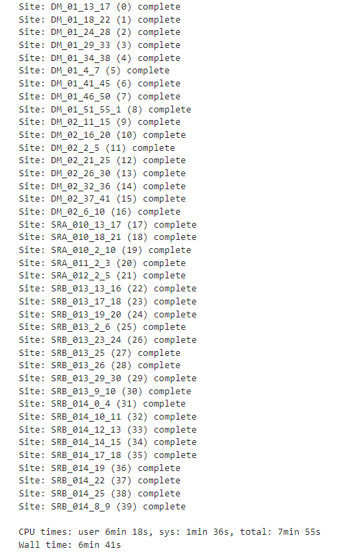
Next, we are going to loop through our field sites:
Clip our dataset using our buffer polygon.
Reproject the clipped data area down to a single reflectance value.
Clipping and reprojecting each clipped area for every time is computationally intensive. We can parallelize the the reprojection process to increase the speed.
%%time

field_data = []
aviris_data = []
for ind, row in gdf.iterrows():

    field_area = ds.rio.clip([row.geometry], all_touched=False)

    def reproj(i):
        return field_area.reflectance.isel(time=i).transpose('wavelength', 'y', 'x').rio.reproject(field_area.rio.crs, shape=(1,1))

    temp = Parallel(n_jobs=4, prefer="threads")(delayed(reproj)(i) for i in range(field_area.time.__len__()))

    temp = xr.concat(temp, dim='time').to_dataset().squeeze().reflectance.values.T[None, ...]
    aviris_data += [temp]

    field_data += [np.asarray(field_data_df.iloc[ind])[...,None].T]

    print(f"Site: {row.unique_id} ({ind}) complete")

print()
field_data = np.concatenate(field_data, axis=0)
aviris_data = np.concatenate(aviris_data, axis=0)
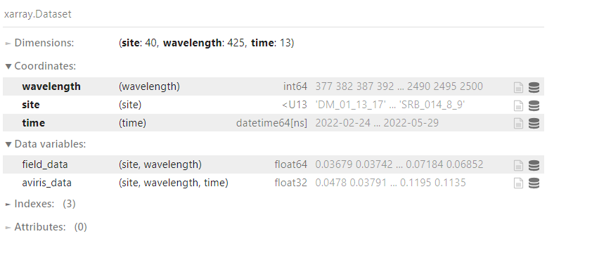
Once we have our data we can use the numpy arrays to create an xarray dataset.
coords = {'wavelength':(['wavelength'], ds.wavelength.values.astype(int)), 'site':(['site'], list(gdf.unique_id)), 'time':(ds['time'].values)}
data_vars = {'field_data':(['site', 'wavelength'], field_data), 'aviris_data':(['site', 'wavelength', 'time'], aviris_data)}

out_ds = xr.Dataset(data_vars=data_vars, coords=coords)
out_ds
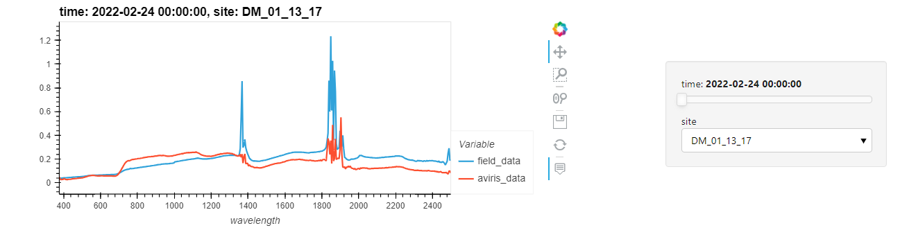
Using the hvplot xarray extension we can plot the field and AVIRIS refelectance for each site and observe how the AVIRIS data compares to the field data at each recording date.
out_ds.hvplot(x='wavelength').opts(xticks=10)